Once you have a workable model, having the right features tend to give the biggest performance boost compared to clever algorithmic techniques such as hyper-parameter tuning. State-of-the-art model architectures can still perform poorly if they don’t use a good set of features.

Learnt features vs engineered features

• The promise of deep learning is that we won’t have to handcraft features.
• However, we’re still far from the point where all features can be automatically learnt.

Feature engineering requires knowledge of domain-specific techniques.

Summary of best practices for feature engineering:

• Split data by time into train/validate/test splits instead of doing it randomly.
• If you oversample your data, do it after splitting.
• Scale and normalise your data after splitting to avoid data leakage.
• Use statistics from only the train split, instead of the entire data, to scale your features and handle missing values.
• Understand how your data is generated, collected and processed. Involve domain experts if possible.
• Keep track of your data’s lineage.
• Understand feature importance in your model.
• Use features that generalise well.
• Remove features that are no longer useful, from your models.
• In most real-world ML projects, the process of collecting data and feature engineering goes on as long as your models are in production.

Common feature engineering operations:

• Handling missing values
  • Not all types of missing values are equal.
  • Missing not at random (MNAR)
    • When the reason a value is missing is because of the true value itself.
    • Example: people with higher income may choose not to disclose their income.
  • Missing at random (MAR)
    • When the reason a value is missing is not due to the value itself, but due to another observed variable.
    • Example: People of some specific gender in a particular survey don’t like disclosing their age.
  • Missing completely at random (MCAR) – (Rare)
    • When there’s no pattern in when the value is missing.
    • There are usually reasons why certain values are missing and you should investigate.
  • When encountering missing values, you can either fill in the missing values with certain values (imputation) or remove the missing values (deletion).
  • Deletion
    • Column deletion
      • If a variable has too many missing values, just remove that variable.
      • The drawback of this approach is that you might remove important information and reduce the accuracy of your model.
    • Row deletion
      • If a sample has missing value(s), just remove that sample.
      • This method can work when the missing values are completely at random (MCAR) and the number of examples with missing values is small, say less than 0.1%.
      • You don’t want to do row deletion if that means 10% of your data samples are removed.
      • Removing rows of data can also remove important information that your model needs to make predictions, especially if the missing values are not at random (MNAR).
      • Removing rows of data can create biases in your model, especially if the missing values are at random (MAR).
  • Imputation 
    • Even though deletion is tempting because it’s easy to do, deleting data can lead to losing important information and introduce biases into your model.
    • Common practices include filling the missing values with the default feature value (if it exists), mean, median or mode (the most common value).
    • Sometimes these methods can cause bugs.
    • Avoid filling missing values with possible values.
    • With deletion, you risk losing important information or accentuating biases. With imputation, you risk injecting your own bias into and adding noise to your data, or worse, data leakage.
• Scaling
  • Before inputting features into models, it’s important to scale them to be within similar ranges. This process is called feature scaling.
  • Min-max scaling
    • x’ = (x – min(x)) / (max(x) – min(x))   -> [0, 1] range
    • x’ = a + (x – min(x))(b – a) / (max(x) – min(x))    -> [a, b] range
  • Standardisation
    • x’ = (x – µ) / σ    -> zero mean and unit variance
  • Log transformation
    • In practice, ML models tend to struggle with features that follow a skewed distribution.
    • To help mitigate the skewness, a technique commonly used is log transformation: apply the log function to your feature.
    • While this technique can yield performance gain in many cases, it doesn’t work for all cases and you should be wary of the analysis performed on log-transformed data instead of the original data.
  • Two important things to note about scaling:
    • It’s a common source of data leakage.
    • It often requires global statistics.
  • During inference, you reuse the statistics you had obtained during training to scale new data. If the new data has changed significantly compared to the training, these statistics won’t be very useful. Therefore, it’s important to retrain your model often to account for these changes.
• Discretisation(Quantisation or binning)
  • It is the process of turning a continuous feature into a discrete feature.
  • The downside is that this categorisation introduces discontinuities at the category boundaries.
  • Choosing the boundaries of categories might not be all that easy.
  • In practice, discretisation rarely helps.
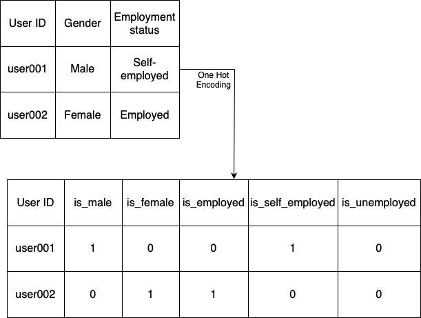
• Encoding categorical features
  • One Hot Encoding
    • Each category is mapped into a binary variable with 0 and 1 as possible values. 0 indicates the absence and 1 indicates the presence of that category.
  • In production, categories change. New categories may appear in production which were not seen in training. These can’t all be put in one category (say “others”) as they are different categories.
  • Hashing trick
    • The gist of this trick is that you use a hash function to generate a hashed value of each category. The hashed value will become the index of that category. Because you can specify the hash space, you can fix the number of encoded values for a feature in advance, without having to know how many categories there will be.
    • One problem with hashed functions is collision: two categories being assigned the same index. However, with many hash functions, the collisions are random. The impact of colliding hashed features is, fortunately, not that bad.
• Feature Crossing
  • Feature crossing is the technique to combine two or more features to generate new features.
  • Because feature crossing helps model non-linear relationships between variables, it’s essential for models that can’t learn or are bad at learning non-linear relationships, such as linear regression, logistic regression and tree-based models.
  • A caveat of feature crossing is that it can make your feature space blow up.
  • Another caveat is that because feature crossing increases the number of features models use, it can make models overfit to the training data.
• Discrete and continuous positional embeddings
  • An embedding is a vector that represents a piece of data.
  • Set of all possible embeddings generated by the same algorithm for a type of data is called an embedding space.
  • Empirically, neural networks don’t work well with inputs that aren’t unit-variance.
  • A way to handle position embeddings is to treat it the way we’d treat word embeddings. With word embedding, we use an embedding matrix with the vocabulary size as its number of columns and each column is the embedding for the word at the index of that column. With position embeddings, the number of columns is the number of positions.
  • Because the embeddings change as the model weights get updated, we say that the position embeddings are learnt.
  • Position embeddings can also be fixed. The embedding for each position is still a vector with S elements (S is the position embedding size), but each element is predefined using a function, usually sine and cosine.
  • Fourier features have been shown to improve models’ performance for tasks that take in coordinates (or positions) as inputs.
• Data Leakage
  • Data leakage refers to the phenomenon when a form of the label “leaks” into the set of features used for making predictions and this same information is not available during inference.
  • Data leakage is challenging because often the leakage is non-obvious.
  • It’s dangerous because it can cause your models to fail in an unexpected and spectacular way, even after extensive evaluation and testing.
• Common causes of data leakage
  • Splitting time-correlated data randomly instead of by time.
    • In many cases, data is time-correlated, which means that the time the data is generated affects its label distribution.
    • To prevent future information from leaking into the training process and allowing models to cheat during evaluation, split your data by time, instead of splitting randomly, whenever possible.
  • Scaling before splitting
    • • One common mistake is to use the entire training data to generate global statistics before splitting it into different splits, leaking the mean and variance of the test samples into the training process, allowing a model to adjust its predictions for the test samples. This information isn’t available in production, so the model’s performance will likely degrade.
      • To avoid this type of leakage, always split your data first before scaling, then use the statistics from the train split to scale all the splits.
      • It’s suggested that we split our data before any exploratory data analysis and data processing, so that we don’t accidentally gain information about the test split.
  • Filling in missing data with statistics from the test split
    • One common way to handle the missing values of a feature is to fill them with the mean or median of all values present. Leakage might occur if the mean or median is calculated using entire data instead of just the train split.
    • It can be prevented by using only statistics from the train split to fill in missing values in all the splits.
  • Poor handling of data duplication before splitting
    • If you have duplicates or near-duplicates in your data, failing to remove them before splitting your data might cause the same samples to appear in both train and validation/test splits.
    • Data duplication can result from data collection or merging of different data sources.
    • Data duplication can also happen because of data processing— for example, oversampling might result in duplicating certain examples.
    • To avoid this, always check for duplicates before splitting and also after splitting just to be sure. If you oversample your data, do it after splitting.
  • Group leakage
    • A group of examples have strongly correlated labels but are divided into different splits.
    • Common for object detection tasks that contain photos of the same object taken milliseconds apart.
    • It’s hard avoiding this type of data leakage without understanding how your data was generated.
  • Leakage from data generation process 
    • Detecting this type of data leakage requires a deep understanding of the way data is collected.
    • There’s no fool-proof way to avoid this type of leakage, but you can mitigate the risk by keeping track of the sources of your data and understanding how it is collected and processed.
    • Standardise your data so that data from different sources can have the same means and variances.
    • And don’t forget to incorporate subject matter experts, who might have more context on how data is collected and used, into the ML design process.
• Detecting data leakage 
  • Data leakage can happen during many steps, from generating, collecting, sampling, splitting and processing data to feature engineering. 
  • Measure the predictive power of each feature or a set of features with respect to the target variable (label). If a feature has unusually high correlation, investigate how this feature is generated and whether the correlation makes sense. It’s possible that two features independently don’t contain leakage, but two features together can contain leakage.  
  • Do ablation studies to measure how important a feature or a set of features is to your model. 
  • Keep an eye out for new features added to your model. If adding a new feature significantly improves your model’s performance, either that feature is really good or that feature just contains leaked information about labels. 
• Engineering good features 
  • More features doesn’t always mean better model performance. 
    • The more features you have, the more opportunities there are for data leakage. 
    • Too many features can cause overfitting. 
    • Too many features can increase memory required to serve a model, which in turn, might require you to use a more expensive machine to serve your model. 
    • Too many features can increase inference latency when doing online prediction, especially if you need to extract these features from raw data for predictions online. 
    • Useless features become technical debts. Whenever your data pipeline changes, all the affected features need to be adjusted accordingly.  
  • In theory, if a feature doesn’t help a model make good predictions, regularisation techniques like L1 regularisation should reduce that feature’s weight to 0. However, in practice, it might help models learn faster if the features that are no longer useful (and even possibly harmful) are removed, prioritising good features. You can store removed features to add them back later, if needed.
  • There are two factors you might want to consider when evaluating whether a feature is good for a model: importance to the model and generalisation to unseen data. 
• Feature importance
  • A feature’s importance to a model is measured by how much that model’s performance deteriorates if that feature or a set of features containing that feature is removed from the model. 
  • SHAP (SHapley Additive exPlanations) is great because it not only measures a feature’s importance to an entire model, it also measures each feature’s contribution to a model’s specific prediction. 
  • Often, a small number of features accounts for a large portion of your model’s feature importance. 
  • Not only good for choosing the right features, feature importance techniques are also great for interpretability as they help you understand how your models work under the hood.
  • InterpretML is a great open source package that leverages feature importance to help you understand how your model makes predictions.
• Feature generalisation 
  • Not all features generalise equally.
  • Measuring feature generalisation requires both intuition and subject matter expertise on top of statistical knowledge.  
  • Two aspects you might want to consider with regards to generalisation: 
    • Feature coverage 
      • Coverage is the percentage of samples that has values for this feature in the data— so the fewer values that are missing, the higher the coverage. 
      • If this feature appears in a very small percentage of your data, it’s not going to be very generalisable. 
      • However, if a feature appears only in 1% of your data, but 99% of the examples with this feature have POSITIVE labels, this feature is useful and you should use it. 
      • If the coverage of a feature differs a lot between the train and test split, this is an indication that your train and test splits don’t come from the same distribution. You might want to investigate whether the way you split your data makes sense and whether this feature is a cause for data leakage.
    • Distribution of feature values.
      • For the feature values that are present, you might want to look into their distribution.
      • If the set of values that appears in the seen data (such as the train split) has no overlap with the set of values that appears in the unseen data (such as the test split), this feature might even hurt your model’s performance.
      • When considering a feature’s generalisation, there’s a trade-off between generalisation and specificity. Example: IS_RUSH_HOUR vs HOUR_OF_THE_DAY features for a model predicting ETAs for a taxi ride. 
      • Feature engineering often involves subject matter expertise and subject matter experts might not always be engineers, so it’s important to design your workflow in a way that allows non-engineers to contribute to the process.