In this section, we talk about how to pre-process and featurise text, image and video data, before it can be passed to an ML model.
Text
Before featurising text into feature vectors, we may need to perform the following pre-processing steps:
- Tokenisation
- This involves breaking down the text into smaller units called tokens. Tokens can be words, subwords or characters, depending on the tokenisation strategy.
- Common tokenisation methods include word tokenisation, subword tokenisation (e.g., Byte-Pair Encoding – BPE) and character tokenisation. For example, the sentence “BERT used to be very popular.” might be tokenised into [“BERT”, “used”, “to”, ” be”, “very”, “popular”, “.”].
- Lowercasing
- Lowercasing helps in ensuring consistency and treating identical words (with different cases) as the same, reducing the vocabulary size and simplifying the learning task for the model.
- Removing punctuation and special characters
- Punctuation and special characters might not always carry meaningful information and could be removed to focus on the essential content.
- Handling numerical values
- We may need to decide how to handle numerical values, whether to keep them as-is, replace them with a placeholder or convert them to text.
- Stop word removal
- Stop words are the most common words in any language (like articles, prepositions, pronouns, conjunctions, etc) and do not add much information to the text. Examples of stop words in English are “the”, “a”, “an”, “so”, “what”.
- Removing stop words that do not contribute much to the meaning of a sentence, can reduce noise and decrease the dimensionality of the feature space.
- The decision to remove stop words from text data depends on the specific task and its goals.
- Handling contractions and abbreviations
- This may help ensure that the model understands the full meaning of words.
- Spelling correction
- Correcting misspellings would likely improve the model’s ability to understand and generate text correctly.
- We could use libraries like “pyspellchecker” or implement algorithms like Levenshtein distance (edit distance) to find the closest words to a misspelled word in a predefined dictionary.
- Handing rare or out-of-vocabulary words
- Rare words might not have sufficient occurrences for the model to learn meaningful representations.
- One way to handle them would be to replace them with a special token.
- Stemming and lemmatisation
- Reducing words to their root form (stemming) or base dictionary form (lemmatisation), can help in capturing the core meaning of words.
- Example of stemming: going -> go
- Example of lemmatisation: better -> good
- Handling emoticons
- It might be a tricky to decide whether to keep or remove emojis as they might carry important sentiment or contextual information.
Featurising text is a critical step in Natural Language Processing and other Machine Learning tasks involving text data. It involves converting raw text into numerical features that can be used for machine learning algorithms. Let’s look at some common text featurisation techniques:
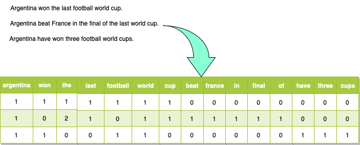
- Bag of Words (BoW)
- This technique represents text data by creating a vocabulary of unique words present in the corpus.
- Each document is then represented as a vector, where each element corresponds to the frequency or presence of a word in the vocabulary.
- The BoW representation ignores the word order and only considers the occurrence or frequency of words.
- TF-IDF (Term Frequency-Inverse Document Frequency)
- TF-IDF calculates the importance of a word in a document relative to the entire corpus.
- It assigns higher weights to words that appear frequently in a specific document but infrequently across other documents.
- TF-IDF combines term frequency (TF) and inverse document frequency (IDF) to create a numerical representation of text data.
- Term Frequency
- TF measures how often a term (word) occurs in a document.

- The idea is that a word is important in a document if it appears frequently.
- Inverse Document Frequency
- IDF measures the importance of a term across a collection of documents.

- The “+1” in the denominator is used to avoid division by zero when a term is not present in any document in the corpus.
- The idea is to give higher weight to terms that are rare across the entire corpus.
- The TF-IDF score for a term in a document is the product of its TF and IDF scores:
- TF-IDF(t, d, D) = TF(t, d) * IDF(t, D)
- The higher the TF-IDF score for a term in a document, the more important that term is in that document relative to the entire corpus.
- N-grams
- N-grams capture the sequential relationship between words by considering contiguous sequences of N words.
- For example, unigrams (N=1) consider individual words, bigrams (N=2) consider pairs of words and trigrams (N=3) consider triplets of words.
- N-grams can be used to capture local contextual information in text data. They can be used with Bag of Words or TF-IDF to featurise text.
- Word Embeddings
- Word embeddings capture the semantic meaning of words by representing them as dense vectors in a continuous vector space.
- Popular word embedding models like Word2Vec, GloVe or FastText learn representations that preserve semantic relationships between words.
- We could use either pre-trained embeddings or embeddings trained ourselves to convert words in the text data into numerical vectors in the following ways:
- Concatenation or pooling
- We could concatenate or pool (e.g., max pooling) individual word embeddings to obtain a fixed-size representation for a document.
- This can capture important phrases or combinations of words.
- Word-level averaging
- In this method, we calculate the average of word embeddings for all words in a document.
- This is simple and effective, but it ignores word order.
- TF-IDF weighted averaging
- Here, we weight word embeddings by their TF-IDF scores to give more importance to rare words.
- Then, we could compute the weighted average of word embeddings for a document.
- Concatenation or pooling
- Contextual Word Embeddings
- Contextual embeddings capture the meaning of words in the context of the surrounding text.
- Models like BERT have achieved state-of-the-art performance in many NLP tasks.
- BERT (Bidirectional Encoder Representations from Transformers) is based on the Transformer architecture, which allows it to capture relationships between words in both directions (bidirectional). This is in contrast to models like Word2Vec, which are unidirectional.
- BERT is pre-trained on large corpora using two unsupervised tasks:
- Masked Language Model (MLM): Predicting masked words in a sentence.
- Next Sentence Prediction (NSP): Determining whether two sentences follow each other.
- In BERT, there is a special token “[CLS]”, which is typically used to obtain a fixed-size representation of the entire input sequence. The output of the [CLS] token is often used as a sentence-level embedding.
- As sentences have variable lengths, we could use pooling strategies (e.g., mean pooling, max pooling) to obtain a fixed-size representation regardless of the input length.
Image
We need to preprocess the images before they can be featurised and used for model training and inference.
- Resizing
- ML models train faster on smaller images and typically require images of the same size. However, real-world images may vary in size, so we need to resize them.
- There are various things to consider when resizing an image like: how small should the resized image be, how to handle square vs rectangular images, maintaining aspect ratio, padding, etc.
- Normalisation
- We could normalise pixel values to a common scale (usually between 0 and 1 or -1 and 1) to ensure consistency and faster convergence during training.
- This can be achieved by dividing pixel values by 255 (if in the range [0, 255]).
- Standardisation (Z-score normalisation)
- Technique to transform data into a standard normal distribution.
- It rescales the data to have a mean of zero and a standard deviation of one.
- If we are dealing with colour images, we need to standardise each colour channel independently by calculating its own mean and standard deviation.
- It helps improve model convergence and generalisation.
- Greyscale
- In many cases, colour is irrelevant for the task. So, converting images to greyscale will reduce the dimensionality and might speed up processing.
- Cropping and padding
- We could crop or pad images to a fixed size if the images have varying dimensions.
- This helps ensure that all images have the same dimensions required by the feature extraction process.
- Data augmentation
- We can apply techniques like rotation, flipping, scaling, shearing or adding noise to increase the diversity of your dataset.
- Data augmentation helps improve the model’s generalisation by exposing it to various versions of the same image.
- Denoising and filtering
- We could remove noise or unwanted artefacts from the images using filters (e.g., median filter, Gaussian filter) or denoising techniques (e.g., bilateral filtering, wavelet denoising) to enhance the quality of the images.
- Histogram Equalisation
- We could improve image contrast and details by applying histogram equalisation, especially in cases where images have uneven lighting conditions.
- Data cleaning
- We may need to detect images of poor quality or corrupted images and handle them properly.
- We could perform integrity checks by verifying file signatures or using checksums (e.g., MD5, SHA-1, SHA-256) to ensure that the file was not corrupted during downloading, storage or transmission.
- We could try using image processing libraries (e.g., PIL, OpenCV) to decode and load the image. Any exceptions or errors raised during the image loading process would indicate image corruption.
- Inspecting pixel values may be helpful here. A value which in not in the expected range would indicate image corruption.
- We could remove the corrupted images from the dataset so that it doesn’t interfere with model training or analysis.
- If the images are important, or there are a lot of corrupted images, we could consider repairing them using these techniques:
- Interpolation: Interpolation methods, such as nearest neighbour, bilinear or bicubic interpolation, can be used to estimate missing or corrupted pixel values by interpolating from neighbouring pixels. These methods work well for small areas of corruption.
- Inpainting: Inpainting algorithms fill in missing or corrupted regions of an image based on surrounding information. Techniques like Patch-based Inpainting, Exemplar-based Inpainting or Neural Network-based Inpainting (using CNNs) are commonly used.
- Median filtering: Median filtering can help in removing salt-and-pepper noise or isolated corrupted pixels by replacing each pixel’s value with the median value in its neighbourhood.
- Imputation: Imputation methods can be used to estimate or impute missing or corrupted pixel values based on statistical measures, neighbouring pixels or similar images in the dataset.
- Error correction codes: For specific types of corruption, error correction codes or techniques can be applied to recover lost or corrupted data bits within an image file.
After image preprocessing, we need to extract features from the images, which can be used for training an ML model or running an inference.
- OCR (Optical Character Recognition)
- OCR converts different types of documents like scanned paper documents, PDFs or images containing text, into text data.
- Before extracting text, we may need to preprocess the input image to enhance text readability. This might involve operations like noise reduction, binarisation (converting to black and white), deskewing (straightening skewed text) and contrast enhancement.
- We could then use OCR tools like Tesseract or GOCR to extract text from the image. This extracted text could then be featurised like any other text.
- Pre-trained Convolutional Neural Networks (CNNs)
- CNNs are powerful deep learning models commonly used for image recognition tasks.
- Pre-trained CNN models, such as VGG16, ResNet or Inception, are trained on large image datasets like ImageNet.
- By utilising these models, we can extract high-level features from the images by passing them through the network’s convolutional layers. These features can be used as image representations for further analysis or classification.
- Image featurisation steps:
- Preprocessing: We’ll need to resize the input images to the required dimensions of the CNN architecture. We could also normalise pixel values to bring them within a certain range (often [0, 1] or [-1, 1]).
- Feature Extraction: We should remove the fully connected layers (top layers) of the pre-trained CNN, leaving the convolutional layers intact. Then, pass images through the network to obtain feature maps or activations from these layers.
- Global Average Pooling: Then, we need to apply Global Average Pooling to the obtained feature maps. This aggregates spatial information, converting each feature map into a fixed-length vector.
- Flattening: We can flatten or concatenate the pooled feature maps to create a high-dimensional feature vector for each image.
- Transfer Learning
- Transfer learning is a technique that leverages pre-trained models on a large dataset and adapts them to a new task with a smaller dataset.
- We can take a pre-trained CNN model and fine-tune it on a labelled dataset specific to our problem.
- By fine-tuning the model’s weights on the new dataset, we can capture image representations that are optimised for our specific task.
- Image Descriptors
- Image descriptors capture low-level visual features of images, such as colour, texture or shape.
- Examples of image descriptors include Histogram of Oriented Gradients (HOG), Scale-Invariant Feature Transform (SIFT) or Local Binary Patterns (LBP).
- These descriptors encode local patterns and characteristics in the image, which can be used as features for classification.
Video
- Frame-Level Features
- We could sample some individual frames from the video and featurise these using image featurisation techniques mentioned above.
- These frame-level features can be aggregated or processed further to obtain video-level representations.
- Optical Flow
- Optical flow is a technique that captures the motion information between consecutive frames in a video.
- It estimates the displacement of pixels between frames, representing the movement of objects in the video.
- Optical flow can be computed using algorithms like Lucas-Kanade or Farneback.
- By analysing the optical flow, we can derive motion-based features that provide information about the dynamics of the video.
- Temporal Pooling
- Temporal pooling techniques aggregate frame-level features over time to create video-level representations.
- Pooling methods such as average pooling or max pooling can be applied to the frame-level features, summarising the information across the video sequence.
- Temporal pooling helps capture global characteristics of the video and reduces the dimensionality of the feature space.
- Recurrent Neural Networks (RNNs)
- RNNs, such as Long Short-Term Memory (LSTM) or Gated Recurrent Unit (GRU), are capable of modelling sequential data.
- RNNs can be used to process the temporal sequence of frames in a video, capturing the dependencies and temporal relationships between frames.
- The hidden states or outputs of the RNN can serve as video-level representations.
- 3D Convolutional Neural Networks (CNNs)
- 3D CNNs extend traditional CNNs by considering spatial and temporal dimensions simultaneously.
- By incorporating 3D convolutions, these networks can directly process video data.
- Pre-trained models like C3D or I3D can be fine-tuned on video data, enabling them to capture spatio-temporal features effectively.